Pythagorean Expectation and Australian Rules Football

I'm a disc sports enthusiast with a data science habit.
Pythagorean expectation, attributed to baseball statistician Bill James is a formula originally used to describe a relationship between the number of runs a baseball team scores and allows, and the team's winning percentage. The basic formula is... (1)
Winning Percentage = (Runs Scored)^2/((Runs Scored)^2 + (Runs Allowed)^2)
For example(2) , the 2002 New York Yankees scored 897 runs and allowed 697. According to the Pythagorean formula they should have won 62.4% of their games, or 101 games. They actually won 103.
Further research has determined that the exponent that better predicts win totals for baseball is closer to 1.83 and varies by sport so an even more general version of the Pythagorean expectation is...
Winning Percentage = (Runs Scored)^k/((Runs Scored)^k + (Runs Allowed)^k)
Scanning the internet, Tony Corke found the following optimal k values suggested:
EPL: 1.3 NHL: 2.15 NFL: 2.37 NBA: 13.91
To this he added 3.87 for AFL (and 1.89 for NRL).
How well did a couple flavors of Pythagorean expectation predict the second half of the 2017 season? I randomly chose 2017 to be my guinea pig...
The plan here is not to evaluate 3.87 as a possible k for AFL. All I'm going to do here is a pandas walkthrough using a k or 2 and a k of 3.87 to look at correlations between the Pythagorean expectation from the first half of the 2017 season and winning percentage in the second half. I'm curious which better predicted teams winning percentages in the last half of the season: winning percentage in the first half, Pythagorean expectation from the first half with 2 as an exponent or Pythagorean expectation with 3.87 as an exponent.
This parallels the assignment at the end of the first week of University of Michigan's online course Foundations of Sports Analytics: Data, Representation, and Models in Sports (via Coursera), which looked at the first and second halves of the 2017-2018 English Premier League season. I follow the same steps taught in that class. I'm using this as an exercise to practice what I've been learning and to begin to play with my new AFL data set from api.squiggle.com.au. (And actually, most of the results of my computations could have been found using this api as well. But I need the practice.)
Away we go...
My starting point is a dataframe called "results_2017" that includes the results of all 207 games of the 2017 AFL season.(3) The first few rows look like this...
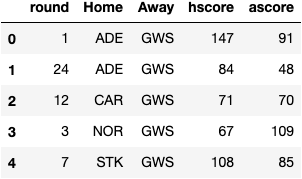
What I'm eventually going to want to have are total wins and losses for each team, and total points for and against for the first and second half of the regular season.
Ah, that's the first problem. This includes finals. Let's get rid of the finals games.
results_2017_rs = results_2017[results_2017['round'] < 24].copy()
Great. We're down to 198 games over 23 rounds.
Now we have to get a count of wins. We'll have to break these into home wins (hwins) and away wins (awins) for now. The 2017 season featured 3 draws, so we're gonna have to count them as 0.5 wins. To get these counts we can use np.where...(4)
results_2017_rs['hwin'] = np.where(results_2017_rs['hscore'] > results_2017_rs['ascore'], 1, np.where(results_2017_rs['hscore'] == results_2017_rs['ascore'], .5, 0))

results_2017_rs['awin'] = np.where(results_2017_rs['hscore'] < results_2017_rs['ascore'], 1, np.where(results_2017_rs['hscore'] == results_2017_rs['ascore'], .5, 0))
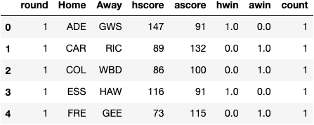
I also just want a count of games. So...
results_2017_rs['count'] = 1
And we're looking at...
Beauty. Now we want to divide the season into two halves (week 12 and before, week 13 and after) and get individual team totals. This will take a few steps.
-Divide dataframe into first and second half of season
-Group by home team and sum all stats
-Rename stats into wins and losses
-Group and rename for home and away, first half and second half. Make 'Team' the index. (four dataframes total)
#split the dataframe chronologically
half1 = results_2017_rs[results_2017_rs['round'] <= 12].copy()
half2 = results_2017_rs[results_2017_rs['round'] > 12].copy()
#group by home team and sum all the stats
hhalf1 = half1.groupby('Home')[['hscore', 'ascore', 'hwin', 'awin', 'count']].sum().copy()
#rename columns ('count' column too. You'll see)
hhalf1.rename(columns = {'hscore' : 'homepointsfor', 'ascore' : 'homepointagainst', 'hwin' : 'homewins', 'awin' : 'homelosses', 'count' : 'hcount'}, inplace = True)
#rename index
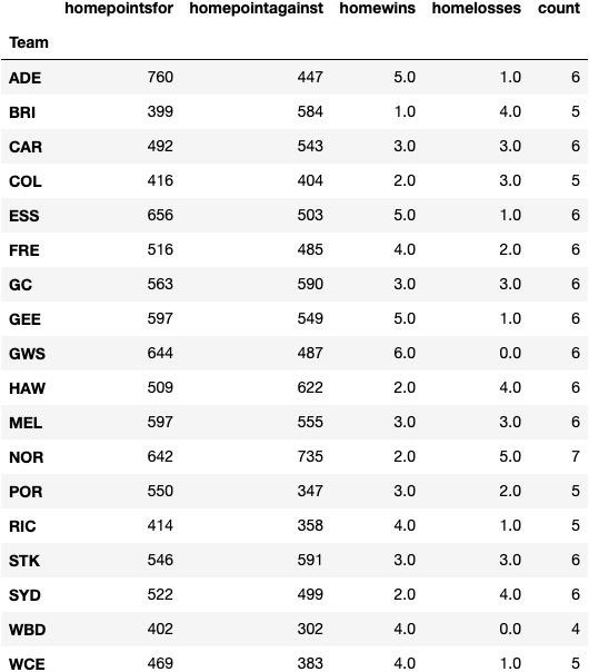
hhalf1.index.name = 'Team'
And then hhalf1 looks like...
Great. Now do this 3 more times: away teams half 1, home teams half 2, and away teams half 2.
ahalf1 = half1.groupby('Away')[['hscore', 'ascore', 'hwin', 'awin', 'count']].sum().copy()
ahalf1.rename(columns = {'hscore' : 'awaypointsagainst', 'ascore' : 'awaypointsfor', 'hwin' : 'awaylosses', 'awin' : 'awaywins'}, inplace = True)
ahalf1.index.name = 'Team'

hhalf2 = half2.groupby('Home')[['hscore', 'ascore', 'hwin', 'awin', 'count']].sum().copy()
hhalf2.rename(columns = {'hscore' : 'homepointsfor', 'ascore' : 'homepointsagainst', 'hwin' : 'homewins', 'awin' : 'homelosses'}, inplace = True)
hhalf2.index.name = 'Team'

ahalf2 = half2.groupby('Away')[['hscore', 'ascore', 'hwin', 'awin', 'count']].sum().copy()
ahalf2.rename(columns = {'hscore' : 'awaypointsagainst', 'ascore' : 'awaypointsfor', 'hwin' : 'awaylosses', 'awin' : 'awaywins'}, inplace = True)
ahalf2.index.name = 'Team'
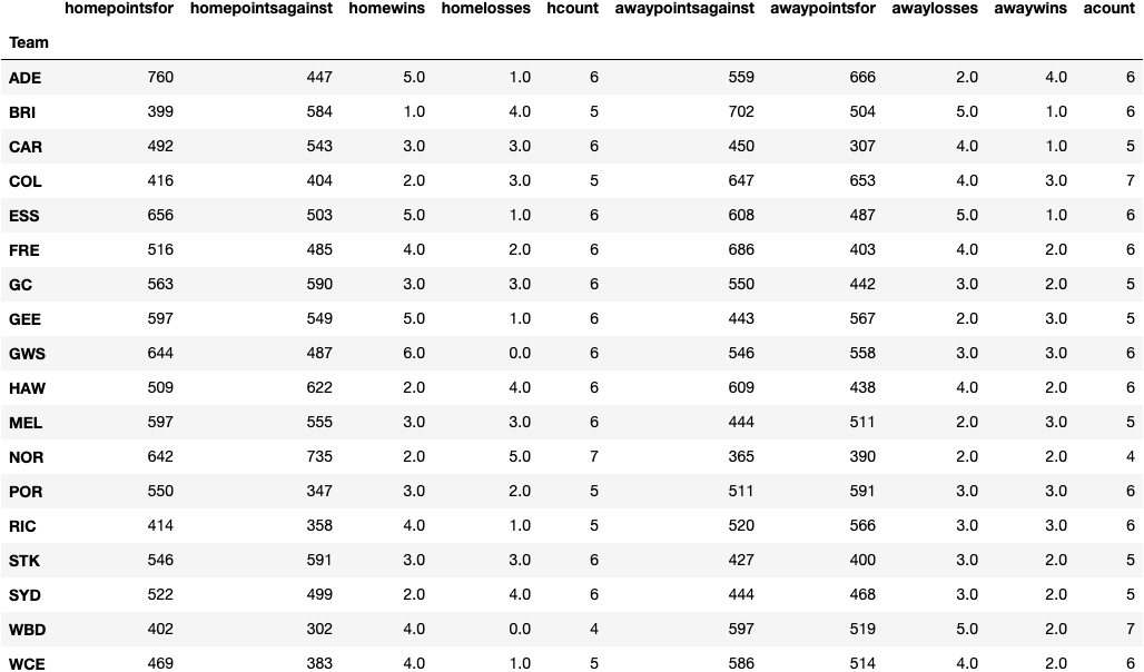
Smashed it. Ok, now to get the team totals for the first and second half. This shouldn't be too hard. First step is to merge the home and away dataframes for each season half based on the team (the index!).```
teams_half1 = hhalf1.merge(ahalf1, left_index = True, right_index = True)
Looking good. Do the same for the second half.
teams_half2 = hhalf2.merge(ahalf2, left_index = True, right_index = True)
Let's add up some columns and get some totals! (we'll figure out their winning percentages too while we're here)
# half 1
teams_half1['W'] = teams_half1['homewins'] + teams_half1['awaywins']
teams_half1['L'] = teams_half1['homelosses'] + teams_half1['awaylosses']
teams_half1['PF'] = teams_half1['homepointsfor'] + teams_half1['awaypointsfor']
teams_half1['PA'] = teams_half1['homepointsagainst'] + teams_half1['awaypointsagainst']
teams_half1['GP'] = teams_half1['hcount'] + teams_half1['acount']
teams_half1['Wpct_half1'] = teams_half1['W']/teams_half1['GP']

#turn down the noise
teams_half1 = teams_half1[['W', 'L', 'PF', 'PA', 'GP', 'Wpct_half1']]

teams_half2['W'] = teams_half2['homewins'] + teams_half2['awaywins']
teams_half2['L'] = teams_half2['homelosses'] + teams_half2['awaylosses']
teams_half2['PF'] = teams_half2['homepointsfor'] + teams_half2['awaypointsfor']
teams_half2['PA'] = teams_half2['homepointsagainst'] + teams_half2['awaypointsagainst']
teams_half2['GP'] = teams_half2['hcount'] + teams_half2['acount']
teams_half2['Wpct_half1'] = teams_half2['W']/teams_half2['GP']

#turn down the noise
teams_half2 = teams_half2[['W', 'L', 'PF', 'PA', 'GP', 'Wpct_half1']]
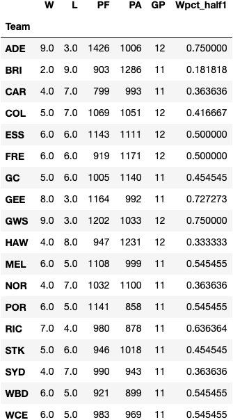
And voila, here's the first half (second half looks similar)...
Now time to get back to ye olde pythagorean expectation (PE). You thought I forgot.
I'm going to compute two different flavors of PE. One with an exponent of 2 ('Classic') and another with 3.87 ('New and Improved'). I'll run both of these for each half season.
teams_half1['CPythE_h1'] = teams_half1['PF']**2/(teams_half1['PF']**2 + / teams_half1['PA']**2)
teams_half2['CPythE_h2'] = teams_half2['PF']**2/(teams_half2['PF']**2 + / teams_half2['PA']**2)
teams_half1['NPythE_h1'] = teams_half1['PF']**3.87/(teams_half1['PF']**3.87 + / teams_half1['PA']**3.87)
teams_half2['NPythE_h2'] = teams_half2['PF']**3.87/(teams_half2['PF']**3.87 + / teams_half2['PA']**3.87)
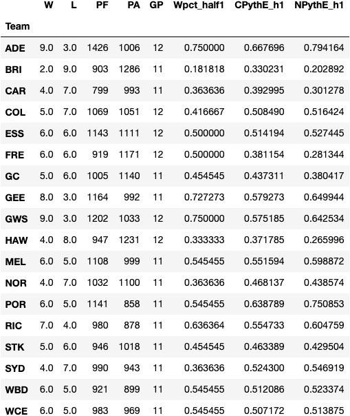
Half 1...
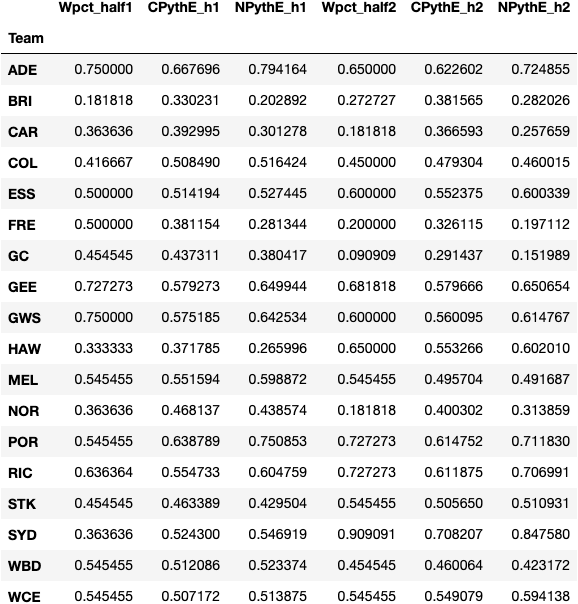
Almost there... now for some summary dataframes...
summary_half1 = teams_half1[['Wpct_half1', 'CPythE_h1', 'NPythE_h1']]
summary_half2 = teams_half2[['Wpct_half2', 'CPythE_h2', 'NPythE_h2']]

# and we merge them...
summary = summary_half1.merge(summary_half2, left_index = True, right_index = True)
And finally we ask our original question again. Which correlates most closely with second half winning percentage: first half winning percentage, PE exponent 2, or PE exponent 3.87? '.corr()' will give us the correlations between variables...
#corr() gives us all the correlations, but we only care about how they correlate with second half winning percentage...

summary.corr()['Wpct_half2']
Wpct_half1    0.412788
CPythE_h1     0.636537
NPythE_h1     0.646018
Wpct_half2    1.000000
CPythE_h2     0.978160
NPythE_h2     0.978490
Name: Wpct_half2, dtype: float64
Of our first half stats, when it comes to predicting second half winning percentage ('Wpct_half2'), 'New and Improved' Pythagorean expectation (exponent 3.87) edged out 'Classic' Pythagorean expectation, and they both solidly beat out first half winning percentage...
(1) I can't find superscript here so I'm using the convention ^ to denote an exponent.
(2) This example and a good overview of pythagorean expectation for a few sports is at Wikipedia .
(3) Of course this isn't really the starting point. I parsed JSON from https://api.squiggle.com.au/?q=games;year=2017 and https://api.squiggle.com.au/?q=teams , created some dataframes, merged them, and prettied it up. If you're unsure how to do this there are many great resources. Use the google.
(4) It's possible that somewhere around here you may come up with a SettingWithCopyWarning. I did. Check out https://pandas.pydata.org/pandas-docs/stable/user_guide/indexing.html#returning-a-view-versus-a-copy for info on this warning. That's where the '.copy()' came from.


