So I was chatting in a Clubhouse room the other day and someone said the craziest thing…

(BTW I love me my Clubhouse)

He said that he had read somewhere that there was actually no home field advantage in football (soccer). There may be some tilting in results toward home teams, but… p-values… not statistically significant… yadayada… This I found hard to believe. I told him that we should crunch some numbers and dedicate a night at clubhouse to the “Myth of the Home Field Advantage.” And here is my first attempt at crunching numbers.

My data is all game results from an NBA data set on Kaggle . It contains over 60,000 games starting from the 1946-7 season. My methodology, hypothesis-testing using permutation resampling methods, comes straight from Datacamp’s Statistical Thinking in Python (Part 2) course. Is this the right situation to be using permutation testing? I’m not sure. I might be overthinking and overcomplicating the issue. Probably, I need the practice though.

My starting point is a question: do home teams score more points than away teams? This question then gets flipped and becomes our hypothesis that we will test: There is no difference in scoring between home and away teams.

THAT’S ABSURD! JUST TAKE THE MEAN! MEAN OF HOME SCORES IS LIKE 105! MEAN OF AWAY SCORES IS LIKE 101! DONE!

The home scores’ mean is higher. That’s a fact. But is it enough of a fact to say that there is a definitive home court advantage? Maybe this is just how the numbers fell. Maybe it could have easily been the away team that ended up with more points. Do we have enough information to strongly rule out that possibility?

Let’s see what happens.

So in this amazing dataset there’s a table with all the game results. It looks something like…

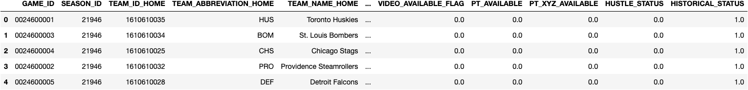
62,448 rows and 149 columns. Awesome.

But really, we only need two columns, home points and away points.

Games = Games[['PTS_HOME', 'PTS_AWAY']]

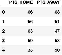
Much better. Now let’s make these two columns into arrays and we’re off to the statistical races…

Home_pts = Games['PTS_HOME']
Away_pts = Games['PTS_AWAY']

To restate our (null) hypothesis, that array of scores by the home team and the away score array are just part of one population of scores, and it just happened that in the games that we’re looking at, the population was divided such that the home teams had more of the higher ones. So that is what we are going to simulate using permutation testing.

Permutation testing is a resampling method which is used to determine whether two samples come from the same population. What we do is mix up (“permute”) the two samples and randomly divide them into two samples. We then take a test statistic that compares the two samples, in our case, for example, we will be using difference of their means. After doing this many times, we will look at the results, the test statistics from all the permutations (“permutation replicates”), and see how many of them are as extreme as the empirical test stat, in our case the observed difference between the home and away scoring means. That will give us an idea of how possible it is that our original home and away samples are actually not so different after all.

Here’s what that looks like as a function…

def draw_DOM_perm_reps(data1, data2, size=1):

    "Draws permutation replicates with difference of means as the function"

    # Concatenate the data sets: data
    data = np.concatenate((data1, data2))

    # Initialize array of replicates: perm_replicates
    perm_replicates = np.empty(size)

    for i in range(size):

        # Permute the concatenated array: permuted_data
        permuted_data = np.random.permutation(data)

        # Split the permuted array into two: perm_sample_1, perm_sample_2
        perm_sample_1 = permuted_data[:len(data1)]
        perm_sample_2 = permuted_data[len(data1):]

        # Compute the DOM
        perm_replicates[i] = np.mean(perm_sample_1) - np.mean(perm_sample_2)

    return perm_replicates

Our function takes three arguments: Two arrays of data and the number of times we want to permute the arrays and take the difference of their means. First, we put the arrays together (“concatenate” them). Then we initialize an array that is going to hold our results. Then, as many times as we have entered as an argument, we will permute the concatenated array, and split it into two new sample arrays. We then take the difference of the means and plug it into our “result” array. Finally, we return the result array.

Ok, then. Let’s go ahead and plug our NBA data into the function and run it, say, 10,000 times.

perm_reps = draw_DOM_perm_reps(Home_pts, Away_pts, 10000)

Now let’s figure out how many of those permutation replicates are as extreme as what we observed as a difference between home and away scoring. That percentage that are as or more extreme is what’s called a p-value. If a lot of the differences of means are as or more extreme than the four-or-so point difference we saw in our observed data, then the p-value will be high, and we will have to think that it is possible that there really is not any home court advantage. A small p-value will tell us that it is likely that home court advantage is real. Let’s see what happens…

# Compute difference of mean scores from our data: empirical_diff_means
empirical_diff_means = np.mean(Home_pts) - np.mean(Away_pts)

# Compute p-value: p
p = np.sum(perm_reps >= empirical_diff_means) / 10000

# Print the result
print('p-value =', p)

p-value = 0.0

Ok. That tells us in none of the 10,000 permutation tests we ran could we find a difference greater than our observed difference. For the hell of it I’m going to run it 100,000 times… five long minutes later…

p-value = 0.0

A million times? I know there are weird permutations out there… c’mon, baby…

74 painful minutes later…

p-value = 0.0

Ok. Did I screw up somewhere? I reran the whole experiment using only the last five seasons of data. With smaller data sets, I was hoping to see some test stats that could surpass our observed difference of means…

p-value = 0.0

OK. Only the last season of data…

p-value = 0.072206

Woohoo! It took us limiting our data to only one out of the NBA’s 74 seasons to come up with permutations with greater differences of means than our empirical findings. In fact, if we were limited to only this one season of data, the p-value surpasses the (kinda arbitrary) 0.05 threshold that signifies to statisticians whether or not findings are “statistically relevant.” This means that with only one season of data, we might say that home court advantage might, actually, not be real.

But we have more data than that. Using just the last five seasons of data (let alone 74), we can argue that there’s less than a one-in-a-million chance that home teams score the same amount as away teams.

Let’s take a look at this graphically.(1)

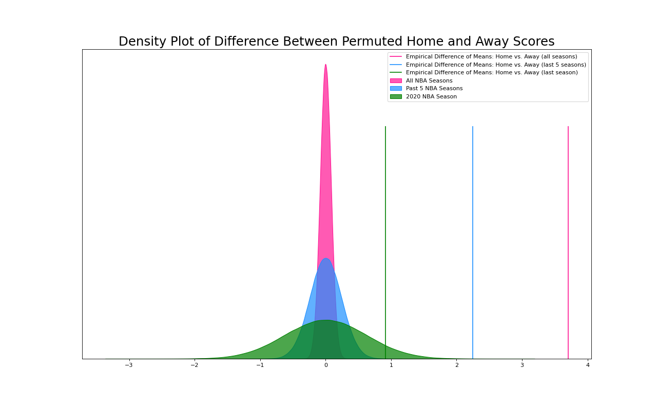
Here I’ve plotted the 1,000,000 differences between the means of the permuted home scores and the away scores for our three arrays, those based on 74 years of data, on five years, and on one year. If we only look at the 2020 data, it looks possible that the empirical difference of means could be part of a randomly generated population that ignores home and away differentiation, i.e. home court doesn’t exist. Two factors, of course, lead to this situation. The smaller dataset naturally has greater variance of the permuted replicates. Secondly, last year had a particularly low empirical difference of means between home and away scores. Home teams only scored ~0.92 points more than away teams. This is far lower than the five year average of ~2.24 points. This one year lack of home court advantage may have been due to so many games being played in empty stadiums due to covid.

When we compare the empirical difference of means to the permutation replicates, we can confidently say that the home team’s scoring advantage could not be arbitrary. That means that in the NBA, home court advantage exists.

---

1. Coding the visualization…

# Create arrays of permutation replicates for the five year data set and the one year data set
# Compute an empirical difference of means for each

Games = pd.read_sql_query("SELECT * FROM Game", conn)
Games = Games[Games['SEASON_ID'].astype('int64') >= 22016]
Home_pts = Games['PTS_HOME']
Away_pts = Games['PTS_AWAY']
perm_reps_5 = draw_DOM_perm_reps(Home_pts, Away_pts, 1000000)
edm_5 = np.mean(Home_pts) - np.mean(Away_pts)

Games = pd.read_sql_query("SELECT * FROM Game", conn)
Games = Games[Games['SEASON_ID'].astype('int64') == 22020]
Home_pts = Games['PTS_HOME']
Away_pts = Games['PTS_AWAY']
perm_reps_1 = draw_DOM_perm_reps(Home_pts, Away_pts, 1000000)
edm_1 = np.mean(Home_pts) - np.mean(Away_pts)

#Create the KDE plot

plt.figure(figsize = (16, 10), dpi = 80)

sns.kdeplot(perm_reps, shade=True, color = "deeppink", label = 'All NBA Seasons', alpha = .7)
sns.kdeplot(perm_reps_5, shade=True, color = "dodgerblue", label = 'Past 5 NBA Seasons', alpha = .7)
sns.kdeplot(perm_reps_1, shade=True, color = "g", label = '2020 NBA Season', alpha = .7)

plt.axvline(empirical_diff_means, color = "deeppink", label = 'Empirical Difference of Means: Home vs. Away (all seasons)', ymax = 0.75)
plt.axvline(edm_5, color = "dodgerblue", label = 'Empirical Difference of Means: Home vs. Away (last 5 seasons)', ymax = 0.75)
plt.axvline(edm_1, color = "g", label = 'Empirical Difference of Means: Home vs. Away (last season)', ymax = 0.75)


plt.title('Density Plot of Difference Between Permuted Home and Away Scores', fontsize=22)
plt.legend()

plt.yticks(ticks = [])
plt.ylabel(None)
#plt.savefig('homecourt_KDE.png')
plt.show()