Do More Possessions Mean More Points in AFL? (A Pandas Walkthrough)

I'm a disc sports enthusiast with a data science habit.
Your first reaction when hearing this question will probably be "of course, duh" (or "What is AFL?". It's Australian Rules Football). You have to think that the team coming away with the ball the most would score the most points in general. With this project I wanted to see if the data supported what seems to be kind of obvious.
The data...
A big part of the reason I decided to take on this project was the amazing dataset that Richard Little ( his twitter ) shared on his github . This data set includes all the play-by-play data (minus six games) from the first 19 rounds of the 2021 AFL season. 683,043 lines of happiness. This is what we're looking at...
Cool huh?
Anyway, here's how this post is going to be structured. I'm going to walk through how I went from that pile of data, to the point that I can make earth-shattering statements about the relationship between number of possessions and points in Australian Football. If you're interested on how I used pandas to move from data to insight, keep on reading. If you are only interested in the punchline, you can skip to the discussion at the end...
Ok. To start at the top. We're going to use pandas. Gotta import it.
import pandas as pd
And we'll use pandas to import the data set.
AFL_PbP = pd.read_csv('AFL Play by play thre r19.csv')
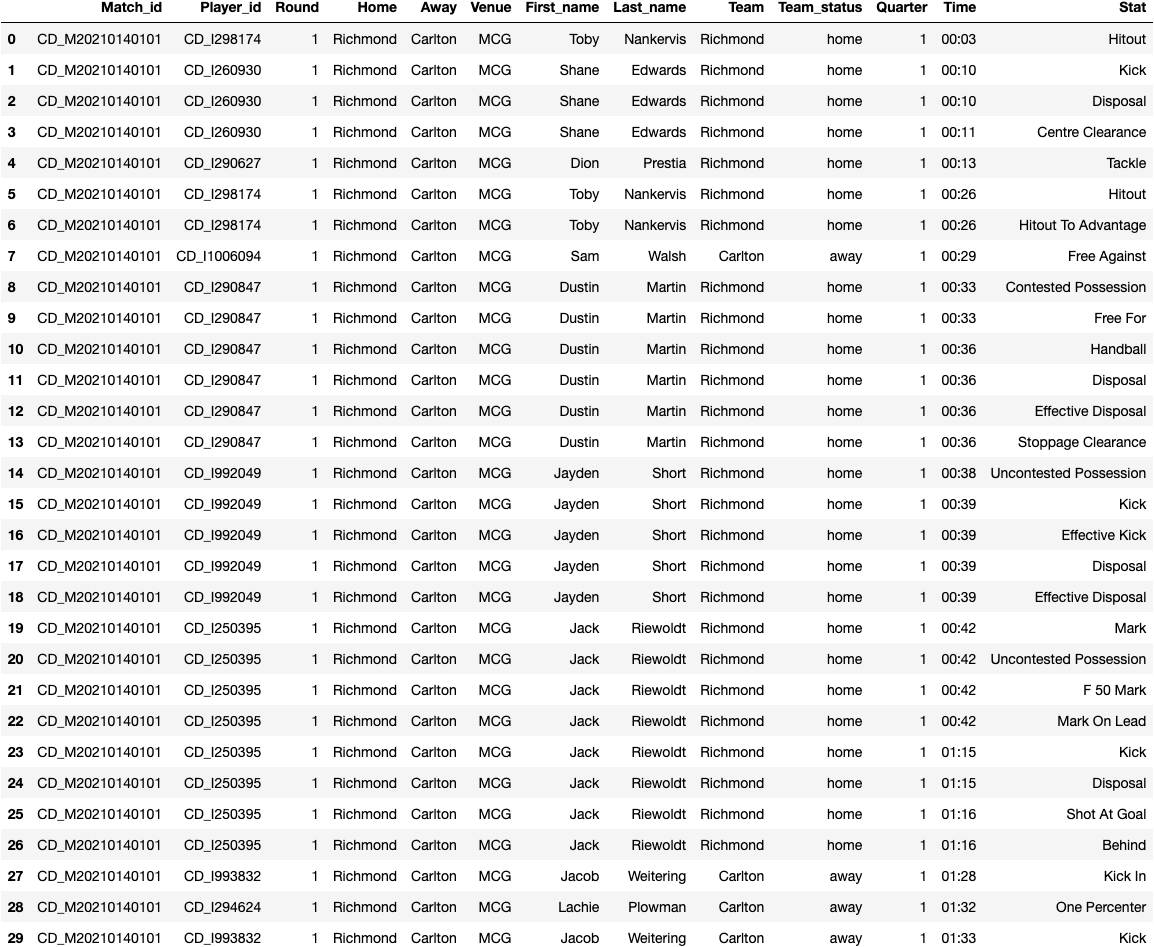
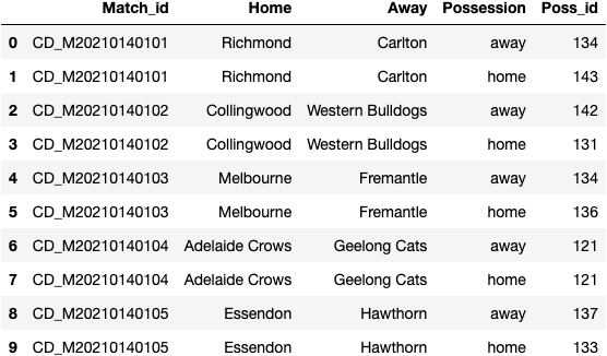
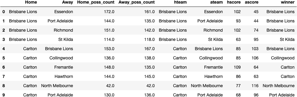
Great. After that I took a look at the top of the data set to get an idea what we were dealing with.
AFL_PbP.head(30)
This gives us the view of the data I showed above.(1)
Next I wanted to take a look at the kinds of stats the dataset recorded. To do that, I made the stat column into a list, and then made that list into a set so I could look at the unique values.
set(AFL_PbP['Stat'].to_list())
{'Behind',
 'Centre Clearance',
 'Clanger',
 'Contested Mark',
 'Contested Possession',
 'Disposal',
 'Effective Disposal',
 'Effective Kick',
 'F 50 Mark',
 'F 50 Tackle',
 'Free Against',
 'Free For',
 'Goal',
 'Goal Assist',
 'Ground Ball Get',
 'Handball',
 'Hitout',
 'Hitout To Advantage',
 'Intercept Mark',
 'Kick',
 'Kick In',
 'Mark',
 'Mark On Lead',
 'One Percenter',
 'Poss Gain',
 'Rebound 50',
 'Running Bounce',
 'Score Launch',
 'Shot At Goal',
 'Spoil',
 'Stoppage Clearance',
 'Tackle',
 'Turnover',
 'Uncontested Possession'}
In the end I want to know how many possessions each team had in each game. Based on the 'stat' and the 'team_status', I needed to figure out where possessions started and ended.
Richard Little, who originally shared the data set, helped me with this guidance: "So possession chains start with poss gain, clearance or kick in. They finish with goal, behind, turnover or stoppage. Stoppage isn't tagged though so you can look for hitout (sometimes doesn't happen) or clearance (and then look back for the time gap)."
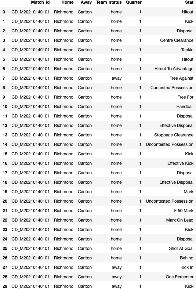
This became my starting point, though needed to be tweaked some as it became code. First, I wanted to get rid of information I was not going to use for this task. So I created a new dataframe with just this data.
poss_per = AFL_PbP[['Match_id', 'Home', 'Away', 'Team_status', 'Quarter', 'Stat']].copy()
Ok. Here's where the story almost ended prematurely. So I wrote out what I thought was some pretty good code to figure out who had possession at any particular time and to give each possession a unique id. I iterated through each line of the dataframe (in the code the dataframe is called 'poss_per_game', I later changed to 'poss_per'. Don't get too distracted by that) to make that happen. Here's the code, don't look at it too closely. It is not actually the code I ended up using...
poss = None
n=0
Poss_id_list = []
for ind, row in poss_per_game.iterrows():

    if ind == 0 or row['Quarter'] != poss_per_game.loc[ind-1, 'Quarter']:
        poss = None
        Poss_id_list.append(0)

    else:

        if row['Stat'] in ['Poss Gain', 'Centre Clearance', 'Stoppage Clearance', 'Kick In', 'Contested Possession']:
            poss = poss_per_game.loc[ind, 'Team_status']
            poss_per_game.loc[ind, 'Possession'] = poss
        if row['Stat'] == 'Hitout':
            poss = None
            poss_per_game.loc[ind, 'Possession'] = poss
        if row['Stat'] == 'Turnover':
            if poss == 'home':
                poss = 'away'
            else:
                poss = 'home
       ...

        elif poss_per_game.loc[ind, 'Possession'] == poss_per_game.loc[ind-1, 'Possession'] or poss_per_game.loc[ind, 'Possession'] == 'score':
            Poss_id_list.append(Poss_id_list[-1])
        else:
            n+=1
            Poss_id_list.append(n)

poss_per_game['Poss_id'] = Poss_id_list
So I went ahead and tried to run this code. I waited. And waited. Cmoooooonnnnn... I know it's a lot of lines of data but you're a computer. You can do this. It couldn't. I waited what felt like 1000 hours (prolly closer to 30 minutes) before I gave up. Maybe this was too much data for my 2013 Macbook Air. I decided to look around for ways to speed up iteration in pandas. I found an article by Satyam Kumar in Towards Data Science that looked at that exact issue. He recommended turning the dataframe into a dictionary and iterating over the dictionary. I gave it a go, I was desperate.
It was very strange. The code took like a minute to run. Kumar saw a 77x speed gain with this method. I have to think the gain was even larger for me. So I wasn't going to have to give up after all.
So here's the code I used to figure out who had possession and create unique ids for each possession. Basically, I created a variable ("poss") that followed who had possession during each line of data, and a list ("Poss_list") that recorded the possessions. I also set a variable ("n") whose values would be the possession ids and a list ("Poss_id_list") of those values.
Basically, the value of the 'Stat' column determines if a possession is starting, remaining the same, or changing. And then separate possessions are marked by changes in the 'Possession' column (which usually holds the value of 'poss').
poss_per_game_dict = poss_per.to_dict('records')

poss = None
quarter = 0
Poss_list = []
Poss_id_list = []
n=0
for row in poss_per_game_dict:
    if row['Quarter'] != quarter:
        poss = None
        Poss_id_list.append(None)
        quarter = row['Quarter']
        row['Possession'] = poss
        Poss_list.append(poss)
    else:

        if row['Stat'] in ['Poss Gain', 'Centre Clearance', 'Stoppage Clearance', 'Kick In', 'Contested Possession']:
            poss = row['Team_status']
            row['Possession'] = poss
            Poss_list.append(poss)

        elif row['Stat'] in ['Hitout', 'Hitout To Advantage']:
            poss = None
            row['Possession'] = poss
            Poss_list.append(poss)

        elif row['Stat'] == 'Turnover':
            if poss == 'home':
                poss = 'away'
            else:
                poss = 'home'
            row['Possession'] = poss
            Poss_list.append(poss)

        elif row['Stat'] not in ['Hitout', 'Hitout To Advantage', 'Poss Gain', 'Centre Clearance', 'Stoppage Clearance', 'Kick In', 'Contested Possession', 'Goal', 'Behind', 'Turnover']:
            row['Possession'] = poss
            Poss_list.append(poss)

        elif row['Stat'] in ['Goal', 'Behind']:
            row['Possession'] = poss
            Poss_list.append(poss)
            poss = None

#possession counter

        if row['Possession'] == None:
            Poss_id_list.append(None)

        elif row['Possession'] == Poss_list[-2] or row['Possession'] == 'score':
            Poss_id_list.append(Poss_id_list[-1])
        else:
            n+=1
            Poss_id_list.append(n)


poss_per = pd.DataFrame(poss_per_game_dict)


poss_per['Poss_id'] = Poss_id_list
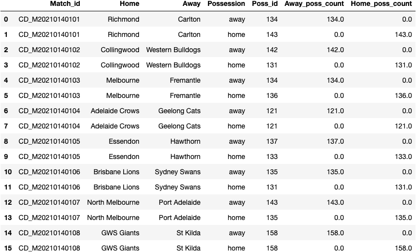
And the result looks like...
pd.set_option('display.max_rows', None)
poss_per.head(50)
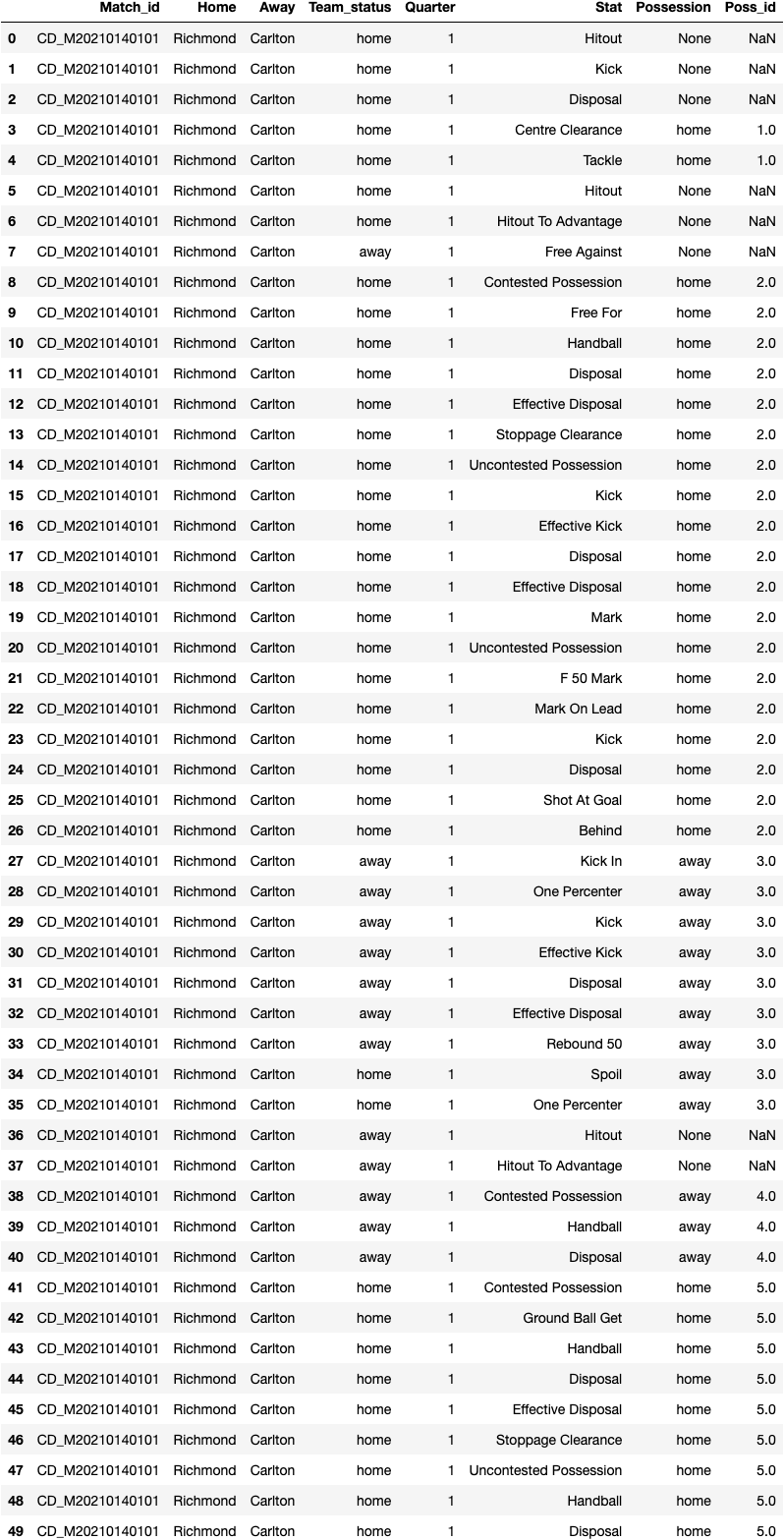
Cool, huh? The Poss_id column has floats but that's no biggie. That was the hard part, now let's get to grouping. First we're going to group by possession. We actually don't care really what happened in the possession, but I took a count of the stats, because, I think I needed to aggregate something.(2)
poss_per = poss_per.groupby(['Match_id', 'Home', 'Away', 'Poss_id', 'Possession'], as_index = False)['Stat'].count()
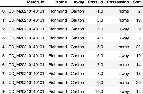
Great. Now we want to count possessions each team had in each game. Let's get to grouping again...
poss_per_game = poss_per.groupby(['Match_id', 'Home', 'Away', 'Possession'], as_index = False)['Poss_id'].count()
I didn't change the name of the column, but 'Poss_id in the above dataframe is the total number of possessions per team per game.
So I would love for there to be just one row per game with columns showing both the home and away possessions. There must be a way to do this by pivoting, but I couldn't find it, so I broke the process up into a couple parts.
for ind, row in poss_per_game.iterrows():
    if row['Possession'] == 'home':
        poss_per_game.loc[ind, 'Home_poss_count'] = poss_per_game.loc[ind, 'Poss_id']
        poss_per_game.loc[ind, 'Away_poss_count'] = 0
    else:
        poss_per_game.loc[ind, 'Away_poss_count'] = poss_per_game.loc[ind, 'Poss_id']
        poss_per_game.loc[ind, 'Home_poss_count'] = 0
And then sum them up...
poss_per_game = poss_per_game.groupby(['Home', 'Away'], as_index = False)['Home_poss_count', 'Away_poss_count'].sum()
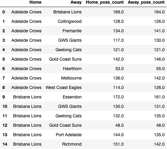
Great. Now we know how many possessions each team had each game. But what was the score? This data set doesn't have that information, but the squiggle api does...
So we're gonna grab the JSON data we want from a url and convert it into something python can read (don't forget to imports requests and json like I always do)...
import requests

url_base = 'https://api.squiggle.com.au/?'
season_url = url_base + 'q=games;year=2021'
response = requests.get(season_url)

import json

data = json.loads(response.text)
If you take a look at 'data', it is a dictionary with one key, whose value is a list of dictionaries, each giving the stats for one game. For example...
data['games'][1]
gives us...
{'hgoals': 14,
 'hscore': 94,
 'winner': 'Sydney',
 'year': 2021,
 'hbehinds': 10,
 'is_grand_final': 0,
 'complete': 100,
 'ateamid': 16,
 'roundname': 'Round 1',
 'ateam': 'Sydney',
 'winnerteamid': 16,
 'ascore': 125,
 'agoals': 19,
 'localtime': '2021-03-20 18:45:00',
 'abehinds': 11,
 'round': 1,
 'date': '2021-03-20 19:45:00',
 'is_final': 0,
 'tz': '+11:00',
 'id': 6245,
 'hteamid': 2,
 'updated': '2021-03-20 22:40:03',
 'venue': 'Gabba',
 'hteam': 'Brisbane Lions'}
All we need are the teams and the scores (though I grabbed the name of the winning team just in case that became convenient). And let's put them together into a dataframe.
hteam = [data['games'][i]['hteam'] for i in range(len(data['games']))]
ateam = [data['games'][i]['ateam'] for i in range(len(data['games']))]
hscore = [data['games'][i]['hscore'] for i in range(len(data['games']))]
ascore = [data['games'][i]['ascore'] for i in range(len(data['games']))]
winner = [data['games'][i]['winner'] for i in range(len(data['games']))]

Season_2021 = pd.DataFrame(list(zip(hteam, ateam, hscore, ascore, winner)), columns = ['hteam', 'ateam', 'hscore', 'ascore', 'winner'])
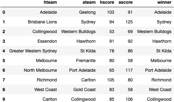
And let's merge this with our 'poss_per_game' dataframe. We know that each team will only play once at another team's stadium, so we can merge on the combination of home team and away team.
combined = poss_per_game.merge(Season_2021, left_on = ['Home', 'Away'], right_on = ['hteam', 'ateam'])
Oh yeah... We're getting close...
(I just dropped the 'hteam' and 'ateam' columns while you weren't looking by the way)
Let's compute the home-away possession ratios and score ratios, because that's what we want to compare (and the difference in the possession count) ...
combined['Home_poss_ratio'] = combined['Home_poss_count']/(combined['Home_poss_count'] + combined['Away_poss_count'])
combined['Home_score_ratio'] = combined['hscore']/(combined['hscore'] + combined['ascore'])
combined['Possession Count Difference'] = (combined['Home_poss_count'] - combined['Away_poss_count']).abs()
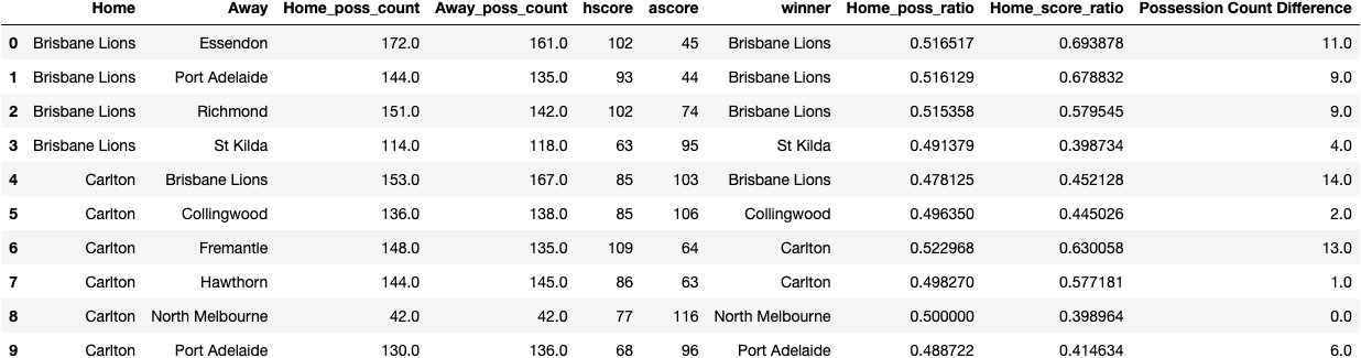
And finally, we can find the correlation between the possession ratio column and the score ratio column.
combined['Home_poss_ratio'].corr(combined['Home_score_ratio'])

#0.6543557079622688
So we see that relative number of possessions is strongly correlated to relative score.
What Does This All Mean?
When I started working with these numbers I came in thinking that the relationship between number of possessions and score would be pretty clear. It wasn't.
The first thing I noticed how thin the possession margins were and how wide the score differences were. Over the time frame discussed the average difference in possessions was 6.21 while teams averaged 130.74 possessions per game. Meanwhile, the average difference in score was 31.67 with teams only averaging 80.53 points per game.(3) It was hard for me to imagine that a few possessions here or there would really relate that strongly to the score. So the 0.6544 correlation between possession ratio and score ratio shocked me. If we plot the games in the dataset, the correlation becomes slightly more obvious.(4)
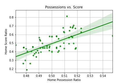
What I find most interesting about this plot is that the x-axis is inching along at 0.01 per gridline. So we can see that the score ratio (and, relatedly, the win ratio) varies greatly just between having 52% of the possessions and 48%.
Obviously, a team that is winning a game is probably winning in a lot of statistical categories, and this is a small dataset, but I did find the results of this exercise interesting. Maybe money spent on a good ruckman is money very well spent.
1. To generate the image of the dataframe and save it as a png I used the dataframe-image library. Install it on your machine or in your notebook and away you go...
import dataframe_image as dfi
dfi.export(AFL_PbP.head(30), 'AFL_Stats_head.png')
2. I really just wanted to group without aggregating, but the output was always a "group-by object", not a dataframe, which was far harder to work with than a dataframe. If I aggregated something, though, the output was a dataframe. I would love some wisdom on this issue. Please drop a comment.
3.
combined['Possession Count Difference'].mean()
(combined['Home_poss_count'].mean() + combined['Away_poss_count'].mean())/2
(combined['hscore'] - combined['ascore']).abs().mean()
(combined['hscore'].mean() + combined['ascore'].mean())/2
4.
import seaborn as sns
import matplotlib.pyplot as plt
sns.regplot(x = 'Home_poss_ratio', y = 'Home_score_ratio', data = combined, color = 'green', scatter_kws={"s": 20})
plt.xlabel('Home Possession Ratio')
plt.ylabel('Home Score Ratio')
plt.title('Possessions vs. Score')
plt.grid()


